Lab 6 - Geometric Correction

Goal and Background

The goal of this particular lab was to introduce us to the very important remote sensing concept of geometric correction of remotely sensed images.  This lab was set up so that we would gain experience with the two major forms of geometric correction, image-to-map rectification and image-to-image registration, and understand the processes of implementing one over the other. 

Methods

Part 1

First, open Erdas Imagine with two separate viewers and put the provided distorted image in one viewer and the provided reference map in the other viewer.  Make sure that the viewer with the distorted image is selected and then click on the Multispectral tab under the raster options and select the Control Points tool.  This will open the Set Geometric Model dialog where you will scroll down and select the option of Polynomial and click OK.  Hitting OK will open up two new tools, the Multipoint Geometric Correction tool and the GCP Tool Reference Setup tool.  On the latter tool, accept the default option Image Layer (New Viewer) and click OK.  Next, navigate to the folder that contains your images and add the reference image and click OK on the Reference Map Information dialog that pops up.  This will then open the Polynomial Model Properties (No File) dialog and accept the default settings by clicking Close.  Next, in the Multipoint Geometric Correction Window, remove any GCP's that were present in the image to begin with and begin adding your own.  Click on the Create GCP tool and add GCP's in similar locations spread evenly across the image to both the reference image and the distorted image for only the first three GCP's.  As this is a first order polynomial transformation only three GCP's are needed for the model solution to be considered current but it is always recommended to collect more than the minimum amount of GCP's.  For the fourth GCP, simply add one to one image and the matching GCP will be added to the other image automatically.  Next, you must reduce the Root Mean Square (RMS) Error to below 2.0 or less, though 0.5 or less is the standard but as this is the first time doing this, 2.0 is more achievable for learning purposes.  Zoom in to the GCP's and move them around on the distorted and reference images until they match up and the RMS Error is within allowable limits.  Once this is done, run the Display Resample Image Dialog and save the output image to the appropriate location and let the too run, dismissing it once it is finished.  You should now have a new geometrically corrected image.

Part 2

For part 2, open Erdas Imagine and bring in the distorted and reference images in the same way you did for part 1.  Next, click on the Control Points button under the Multispectral tab as you did in part 1 and once again select Polynomial under the Set Geometric Model dialog and click OK on the GCP Tool Reference Setup tool.  Import your reference image and then click OK on the Reference Map Information dialog.  On the Polynomial Model Properties dialog change the Polynomial Order from 1 to 3 and click Close.  Next, click on the Create GCP tool and add in 9 GCP's to both images in a similar location and then add 3 more to just one of the images in a similar way to what was done in part 1.  Move the GCP's around until you get an RMS Error of below 1.0 in this case and once this is achieved, run the Display Resample Image Dialog and save the output image in the necessary folder.  Make sure to change the Resampling Method to Bilinear Interpolation under the Resample Image Window and keep all of the other default settings and then click OK to run the tool.  After the tool is completed, you will have a geometrically corrected image using a third order polynomial with bilinear interpolation.  

Results

Part 1 Multipoint Geometric Correction Window with 4 GCP's and an RMS error of .9721

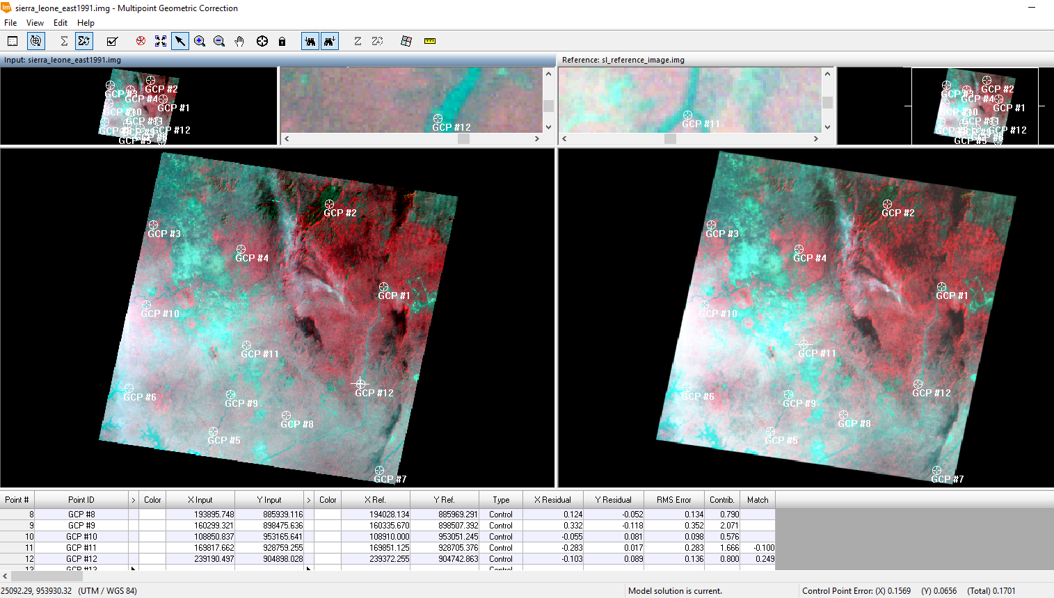
Part 2 Multipoint Geometric Correction Window with 12 GCP's and an RMS error of .1701

Sources

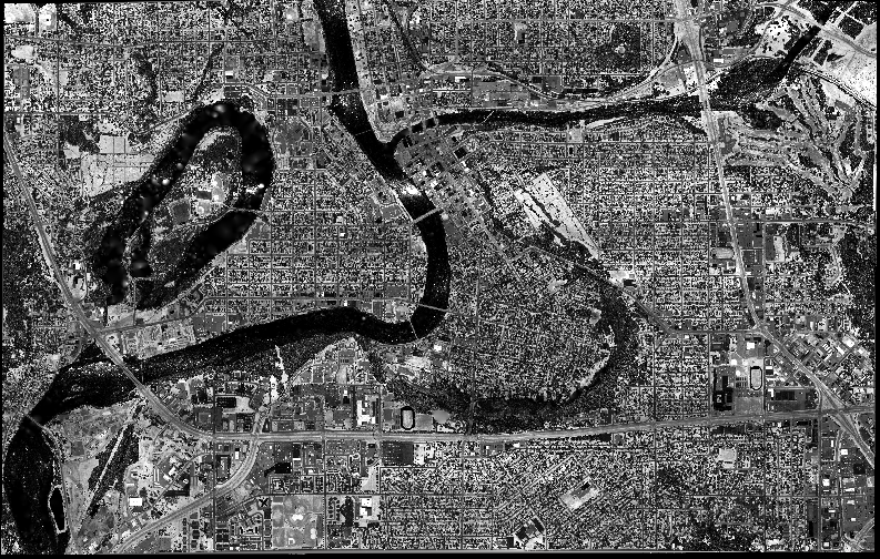
Satellite images are from Earth Resources Observation and Science Center, United States Geological Survey.

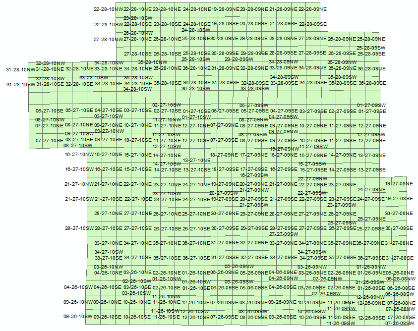
Digital raster graphic (DRG) is from Illinois Geospatial Data Clearing House.

Lab 5 - LiDAR Remote Sensing

Goal and Background

The goal of this lab was to begin to develop a basic knowledge of LiDAR data and its fundamental formats and uses. This lab tested our ability to analyze and interpret LiDAR data in a variety of ways as well as taught us the basics of using ArcMap and Erdas Imagine functions to develop different ways of viewing and analyzing the data.  The primary ways of developing these skills was through the creation and processing of various terrain and surface models as well as an intensity image from point cloud.

Methods

Part 1: Point cloud visualization in Erdas Imagine

Using the files provided by the professor, the first step to demonstrate LiDAR data was to open a new Erdas Imagine viewer and add in all of the LAS as Point Cloud (.las) files, making sure to click NO on the LOD warning screen that will appear. Next, to check the location of the .las tile, open ArcMap and load the provided shapefile of the study area, QuarterSections_1.shp and use the label field Quarter_1 to locate a particular .las file's tile position on the tile index shapefile that is opened in ArcMap.  For the majority of the rest of this lab, ArcMap will be used as it is easier to process lida point clouds.

.las files in Erdas Imagine

QuarterSections_1.shp shapefile with labels based on each block

Part 2: Generate a LAS dataset and explore lidar point clouds with ArcGIS

Using the provided .las files once again, open ArcMap and navigate to the ArcCatalog.  Once there, navigate to the folder with all of the .las files and right click, selecting New>LAS Dataset.  Name the new dataset  Eau_Claire_City and right click on it in the ArcCatalog to open its LAS Dataset Properties window. Next, click on the add data button and add all of the .las files and then go to the Statistics tab and hit the Calculate button.  Next, coordinate systems must be added and to find out which ones to add, go to the metadata .xml file for the data and open it in notepad and find the horizontal and vertical coordinate systems.  In this case, we will use the  NAD 1983 HARN Wisconsin CRS Eau Claire (US Feet) for the horizontal and NAVD 1988 US feet for the vertical.  Navigate to these coordinate systems for both the XY Coordinate Systems tab and the Z coordinate system tab and select and apply them.  Next, put the properly formatted LAS Dataset into the ArcMap window by dragging the created Eau_Claire_City.lasd into the window.  Right click the layer in the TOC and go to its properties and classify it with 8 instead of 9 classes.  Using the LAS Dataset toolbar, play around with the different surface options from the Surface drop down menu such as Aspect, Slope, and Contour.

Aspect Surface

Contour Surface

Slope Surface

With the Contour surface selected, right click on the Eau_Claire_City.lasd layer and go to its properties.  Here you can adjust the contour interval as well as other settings. Next, go to the filters tab and view the differences between the different predefined settings like All (default), Ground, Non Ground, and First Return and pay attention to the differences in what classes and/or returns each different setting uses.

Next, return to the full extent view and set the points to Elevation and the filter to First Return.  then, go to the LAS Dataset toolbar and select the  LAS Dataset Profile View tool.  Find a object on the map that you know the shape of, in this case an old rail bridge now used as a pedestrian bridge to downtown, and use the tool to create a box around the object to display it.

Part 3: Generation of Lidar derivative products

Section 1: Deriving DSM and DTM products from point clouds

First, open the ArcToolbox and navigate to Conversion Tools > To Raster > LAS Dataset to Raster and launch the LAS Dataset to Raster tool. It should look like this.

Input your LAS Dataset and give it the necessary name.  Set the Value Field as Elevation, the Cell Type to Maximum, the Void Filling to Natural_Neighbor, the Sampling Type to Cellsize, and the sampling value to 6.56168 which is equal to 2 meters and then click OK to run the tool.  Next. activate the 3D Analyst extension is active by going to  Customize > Extensions > 3D Analyst.  Then in ArcToolbox go to 3D Analyst Tools > Raster Surface > Hillshade to launch the Hillshade tool.

Input the Digital Surface Model (DSM) you created in the the previous steps and run the tool to create a hillshade of the DSM. 

To create a Digital Terrain Model (DTM), you will use the same LAS Dataset to Raster tool but instead of setting the filter to First Return, you will set it to Ground. Input the LAS Dataset and set the Interpolation to Binning, the Cell Assignment Type to Minimum, the Void Fill method to  Natural Neighbor, the Sampling Type to CellSize, and the Sampling Value to the same 6.56168.  Run the tool to create the DTM.  Next, run the Hillshade tool again in the same way as before but input the DTM instead.

Section 2: Deriving Lidar Intensity image from point cloud

To create an intensity image, set the LAS Dataset to Points and the Filter to First Return before running the LAS Dataset to Raster tool. Set the Value Field to Intensity, Binning Cell Assignment Type to Average, Void fill to Natural Neighbor, and Cell Size to 6.56168.  Run the tool to create the intensity image and then export the image as a TIFF file to be opened in Erdas Imagine for viewing.

Results

Digital Surface Model (DSM) with first return

Digital Terrain Model (DTM)

Hillshade of DSM

Hillshade of DTM

LiDAR Intensity Image of Eau Claire, WI

Sources

Lidar point cloud and Tile Index are from Eau Claire County, 2013. Eau Claire County Shapefile is from Mastering ArcGIS7th Edition data by Margaret Price, 2016.